A video that I made to try and explain mark-release-recapture experiments for mosquitoes. As discussed in this other post, mark-release-recapture experiments are a way of estimating aspects of mosquito ecology, for example, their life expectancy or the distance they disperse. The above video illustrates the way in which these experiments are designed: a number of mosquitoes are marked (typically with a fluorescent dye) and released; on subsequent days mosquitoes are captured and the numbers of marked mosquitoes present in the collection recorded. The faster the rate of decline in the number of captured mosquitoes, the faster the mosquitoes are dying (illustrated by those mosquitoes that turn red above) and/or flying out of the experiment boundaries. Whilst quite a ‘low-tech’ approach, MRR experiments remain one of our most important methods for understanding wild mosquito populations.
Malaria prevalence in Sub-Saharan Africa since 1900
The above video is derived from supplementary data in, “The prevalence of Plasmodium falciparum sub-Saharan Africa since 1900″, Nature, Snow et al., 2017.
Tracing the origins of the HIV pandemic: from chimps into Kinshasa
I recently read `The Origins of AIDS‘ by Jacques Pepin that completely changed the way I view the pandemic of HIV/AIDS. This painstakingly researched book uses a rich palette to paint a detailed picture of the path of HIV. It takes us from its origins in chimpanzees, its transmission into a human hunter in the DRC in the early twentieth century, its subsequent spread through the region riding on the back of a wave of societal transition away from colonial rule, coupled with a paternalistic western-doctor-initiated mass public vaccination program against sleeping sickness. In discussing this journey we meet a diversity of actors who take turns to play roles in the amplification and dissemination of HIV from a local African epidemic to its current worldwide endemicity. They range from prostitutes in Kinshasa, pitifully-cruel colonial administrators, (their replacement) African demagogues, idealistic post-colonialist medics, Haitian blood traders, and homosexuals in California.
Partly because I have recently started to do some really exciting work on HIV with Nico Kist and Astrid Iversen at WIMM in Oxford, I decided that I would make a series of posts about the content of the book. I am under no illusion, this website is mostly just a way for me to keep a record of things I’ve read, and (hopefully) once, understood. However if you find yourself here by serendipity or happenstance or most-likely misfortune, then feel free to read on! I would really recommend reading the book though (can be bought from Amazon here) — it’s fantastic and really opened my eyes about the origins of HIV — and my short clumsy prose are not in any way a substitute for this experience. (Reassuringly, another Ben Lambert pointed this out in the comments below and I couldn’t agree more with their criticism.)
This series of posts are mainly about the most common and virulent form of HIV, known as HIV-1, which accounts for the majority of worldwide infections. This contrasts with another strain of the disease known as HIV-2 which is mostly confined to West Africa, and is the much less virulent of the two strains. This reduced virulence manifests with reduced transmission rates, a slower course of infection, and a delayed passage to AIDS.
In this post I am going to discuss where and how it is believed the disease first successfully crossed into humans. Chimpanzees are our closest relatives, sharing some 99% of our DNA. There are two main species of chimps: Pan troglodytes, the common chimpanzee, and Pan paniscus, the bonobo. However it is now recognised on the basis of mitochondrial DNA that four subspecies exist including, P.t. versus, P.t. ellioti, P.t. troglodytes, and P.t. schweinfurthii that inhabit fairly geographically distinct areas.

Map showing the ranges of the chimpanzee subspecies (by colour) with the territories of two gorilla species indicated. Figure reproduced from, `The evolution of HIV-1 and the origin of AIDS’, Sharp and Hahn, Royal Society B, 2010.
The geographic distribution of chimps corresponds well with the believed epicentre of the HIV-1 epidemic, around the central African countries (the two Congos, the CAR, Gabon, Cameroon and Equatorial Guinea). We have reason to believe that this region is the origin of the epidemic by considering the geographic variation in genetic diversity of the HIV-1 virus. According to Pepin, `HIV-1 evolves at a rate about 1 million times faster than that of … DNA’, meaning that after its introduction into the human population, the virus should rapidly spawn offspring of increasing divergence from the original strain. This trend from one form of HIV-1 to a diversity of HIV-1 variants means that we can use strain diversity as a genetic clock to roughly gauge the age of a particular strain.

Reproduced from, `Genetic diversity of HIV in Africa: impact on diagnosis, treatment, vaccine development and trials’, Peeters et al., AIDS, 2003.
The above map displays as pie charts the diversity of HIV-1 forms from samples collected from across the African continent. From this map it is evident that the greatest geographic diversity in HIV-1 exists in the central African region. Furthermore using data at the city level, researchers have found that the diversity of HIV-1 strains in Kinshasa `twenty-five years ago was far more complex than among strains currently found in any other parts of the world!’. More recently using samples from Congo-Brazzaville in the Republic of Congo, researchers have found similar levels of genetic diversity there (see `HIV-1 subtypes and recombinants in the Republic of Congo’, Niama et al., Infection, genetics and evolution, 2006). These results strongly point to the two Congos as being the starting point for the HIV-1 epidemic.
Comparing the two maps above we see a correspondence between the habitat of P.t. troglodytes and the region of high genetic diversity of HIV-1 strains. Is this a red herring, a mere plot twist to confuse the Poirots of epidemiology? Not one bit of it. This becomes clear when we introduce another actor known as simian immunodeficiency virus (SIV), a type of virus similar to HIV-1 whose symptoms include persistent infections in a number of non-human primates, not uncharacteristic of AIDS in humans. Could it be that HIV-1 is actually derived from SIV?

The phylogenetic relationships between strains of SIVcpz (black from P.t. troglodytes, grey from P.t. scweinfurthii), SIVgor (blue) and subtypes of HIV-1 (red). The red crosses indicate four branches on which cross-species jumps to humans may have occurred; the two blue crosses indicate alternative possible branches on which chimpanzee-to-gorilla transmission may have occurred. Reproduced from, `The evolution of HIV-1 and the origin of AIDS’, Sharp and Hahn, Royal Society B, 2010.
The above graph shows a phylogeny that estimates the evolutionary relationship between HIV-1 subtypes and various subtypes of SIV. In particular this shows that many of the HIV-1 subtypes are more related to their SIV counterparts than they are to their compatriot HIV-1 viruses! In particular considering HIV-1/M ,which is by far the most common subtype of HIV, we find that this virus is more similar to strains of SIVcpz (cpz = chimpanzee) than it is to HIV-1/N, and HIV-1/O. This hints that there are shared evolutionary history between HIV-1 subtypes and subtypes of SIV, and also suggests that there may be a number of cross-species transmissions that initiated the current HIV-1 pandemic.
But questions remain. How did these transmissions occur? And more pertinently since we are proposing a number of these cross-species events, why didn’t these transmissions occur previously and unleash an earlier wildfire of HIV-1?
Using spectroscopy and machine learning to estimate mosquito lifespans
 determines whether a disease spreads over time


Restating the importance of knowing how long wild mosquitoes live
As I said in this post, we need to have better understanding of how long wild mosquitoes live. This would allow us to develop more accurate predictive models of the epidemiology of malaria, as well as other mosquito-borne diseases.
The predominant method used to estimate how long wild mosquitoes live is mark-release-recapture experiments (explained in this post.) These experiments are costly, both financially as well as in terms of time, and effort. Also, factors outside of the experimenter’s control, particularly weather, can cause wild variation in estimates of mosquito longevity. All of these issues with mark-release-recapture methods motivated the meta-analysis which I discussed previously.
Is there another way?
In 2009, a paper was published that showed that a type of spectroscopy, which measured the absorption of infrared light, could be used to predict adult mosquito age (Mayagaya et al., 2009). To estimate mosquito age, the authors started by shining infrared light through individual mosquitoes using an infrared spectroscopy machine like the one below.

Taken from Sikulu et al., (2011), Malaria Journal.
The authors used the above machine to measure how much light was absorbed, or reflected, across a range of wavelengths in the infrared part of the spectrum. Since the mosquitoes were reared in the lab, their age was known. As mosquitoes age there are changes in the mosquitoes’ chemical composition. Since different molecules absorb infrared light to differing degrees, the changes in the mosquitoes’ body chemistry causes differences in the spectra. However, these changes are subtle, meaning that the differences in the spectra are hard to see by eye. The difficulty in detecting these changes is made even harder due to the fact that there is quite a lot of inter-mosquito variation in spectra, as this next figure demonstrates.

The above figure shows a few examples of spectra drawn from a larger data base that we have compiled of the results of these experiments. In the figure there are 34 spectra. Each spectrum (coloured line) shows the result of an experiment on a single mosquito of known age. To try to identify patterns I have coloured each spectrum according to the age of the mosquito at the time of the experiment. For me, I find it difficult to see much of a pattern here. However, fortunately, there are methods that are more sensitive than my eyes!
Machine learning
Whilst it is difficult to visually detect any changes in spectra as mosquitoes age, statistical methods are more adept at these types of problem. In general, statistical methods are used when we want to isolate a ‘signal’ of interest, from a dataset that is noisy. This noise is due to the multitude of factors that can influence the result of an experiment, which are not of direct interest to the experimenter. In this case, as well as the changes in the spectra with age (the ‘signal’), the spectra also vary for a sample of mosquitoes of the same age. This unwanted variability (the ‘noise’) is due to differences in mosquito biochemistry, which are the result of different life histories, genetics, or experimental methods, for example. We would like whichever statistical method we choose to use to be able to see through this noise, and extract out the signal of interest. In this case, we want our statistical algorithm to be capable of estimating the age of individual mosquitoes from their noisy spectra, with a high degree of accuracy.
The experimenters chose to use a ‘Partial Least Squares’ algorithm for this task. This method works by trying to identify linear combinations of input (in this case, the spectra themselves) and output (age) variables, that are most highly correlated. I created the diagram below to try to graphically illustrate how this statistical method works.
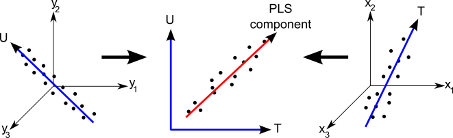
Whilst in this case there is only a single output variable, age, Partial Least Squares can be used to predict a range of output variables. Because of this, in the above figure I show a three dimensional output (the left hand plot), and three dimensional input (the right hand plot.) In our case there are 2,500 input variables, but this is hard to visualise, so in the above figure I just went for three variables. Here T and U illustrate the new variables that are created, from the input and output variables respectively. These variables are constructed so that their correlation with one another is as high as possible (illustrated in the middle plot.)
Results
The Mayagaya et al., (2009) authors calibrated a Partial Least Squares model using spectral data for over 250 observations of mosquito-age. This calibrated model was then used to estimate the age of a set of mosquitoes from their individual spectra. Importantly, these were different mosquitoes from those that were not used to calibrate the original model. Because these mosquitoes were not used to estimate the model, its performance on these ‘test’ set can be regarded as a fairly independent measure of its capability. The graph below shows the actual age versus the predicted for this test set.

Taken from Mayagaya et al., (2009), The American Journal of Tropical Medicine and Hygeine.
In the above figure each dot represents a mosquito at a particular age. The squares indicate average predictions for each of the real age groups. The points are arranged vertically because the mosquitoes were scanned at intervals of exactly three days: from an age of one day, to an age of nineteen days.
The results are quite extraordinary. It still amazes me how this indirect method is able to estimate the age of mosquitoes with any degree of accuracy. That it works at all is testament to the great efforts of the researchers involved.
Can we do better?
However, the predictions aren’t perfect. At younger ages there is a lot of variability. At higher ages, the predicted ages significantly understate the actual age. Are these results good enough for the original purpose of undertaking the research?
Remember, the original reason for undertaking this method was because knowledge about how long mosquitoes live in the wild is very important for understanding the epidemiology of mosquito-borne diseases. In the case of malaria, the impact of the disease on human populations is especially dependent on the age of mosquitoes. This is because mosquitoes must survive the extrinsic incubation period (see this page for a short explanation of this concept) to be able to transmit malaria. Whilst the length period depends on temperature, and possibly on mosquito species, a rough estimate of its duration is 9-12 days. So mosquitoes need to live at least this long to be able to transmit malaria. In reality they will need to be older, since they first have to find a mate, then subsequently bite an infected human. Therefore, perhaps it is more realistic to suppose that mosquitoes must live for at least 10-13 days in order to be able to pass on the disease. Thus, whether malaria spreads through a region, or dies out, depends crucially on the age-structure of the population, particularly whether enough mosquitoes live longer than about 10 days.
The results above indicate reasonable predictive capability for younger mosquitoes, however they also demonstrate that the method falls down for older specimens. However, from the previous discussion, it is precisely these mosquitoes whose age we need to determine! If there are a lot of very old mosquitoes (20 days plus, for example) in a particular region, then malaria will spread much more easily. This also highlights why insecticide-treated bed nets, and other methods that aim to suppress adult mosquito populations, are so effective: they reduce the number of mosquitoes that live long enough to transmit malaria.
So, we need to do a bit better. The research of the authors is a good start, but we need to build on their success.
Our approach
Thomas Churcher at Imperial and I, together with our research collaborators Maggy Sikulu, and Floyd Dowell, have been working towards improving the use of this technology. We started by amassing a data base, of over 5,000 individual spectra. Each of these spectra corresponds to a particular mosquito sample, whose age is known. The data come from a variety of sources, at a range of different laboratories. By using this data we aim to build a statistical model that is robust to variation in experimental technique, as well as geographic variation in mosquitoes.
We have used cutting-edge machine learning techniques, to build a tool that can accurately predict individual mosquito age. The results of this research are promising. The below figure illustrates the predictions made by our machine learning algorithm across approximately 1,000 independent mosquito samples.

In the above figure, the black dots represent individual samples, and the orange line shows the optimal case (actual=predicted). The dark blue line (mostly obscured by the orange) represents our average model prediction at each value of mosquito age, and the blue shading indicates 95% predictive intervals for our algorithm.
These results illustrate that we have removed many of the undesirable features from the results of the original paper: there is reasonable prediction of mosquito age across the entire range that we surveyed. The average predictive error is about 2.5 days. This means that about 70% of our predictions lie within the interval: 


We’re pretty pleased with these results and are currently in the midst of finishing our paper for submission. Along with the above results, in the paper we demonstrate that the use of our algorithm could be used to infer demographic parameters for mosquito populations. All in all it’s quite exciting. After the paper is (hopefully) accepted, I will post more of the results here.
Estimating how long wild mosquitoes live
The lifespan of wild mosquitoes determines the prevalence of malaria
The length of time that adult mosquitoes live determines how easily malaria can spread through a human population. The longer a female mosquito lives (only the females bite), the greater the chance of them biting an infected human host, and becoming infected with the parasite themselves. Within the mosquito the parasite undergoes a complex cycle of life stages, where it transforms itself, and migrates from the mosquito gut to the salivary glands. The whole process takes around 10 days, and is called the extrinsic incubation period. Only once it has arrived in the salivary glands can the parasite be passed to a human, the next time the mosquito blood feeds. If mosquitoes live longer, it is more likely they will survive the extrinsic incubation period, and go on to bite an uninfected human; passing on the disease.
Our current understanding of how long mosquitoes live in the wild is poor
Whilst it is important to know how long adult mosquitoes live in the wild, currently this aspect of mosquito ecology is poorly understood. The primary method for estimating mosquito lifetimes are mark-release-recapture experiments. In these experiments, mosquitoes are either reared in a lab, or captured from the wild. They are then marked, typically using a fluorescent dust, and released into the wild. By monitoring the number of marked mosquitoes that are recaptured over time this allows us to estimate the combined rate at which mosquitoes die, and migrate away from the study area.

The above figure shows example results from two hypothetical mark-release-recapture experiments, where 1,000 marked mosquitoes were released (on day 0). The mosquitoes were recaptured on even days following release, for two different mosquito populations: one with a long lifespan and/or a slow migration rate (blue dots); another with a relatively short life expectancy and/or a faster rate of migration out of the study area (orange).
These experiments aren’t perfect, and outside factors can affect the number of mosquitoes that we actually recapture on a given day. Because of these random factors that we can’t control, we use statistical techniques to account for them, and estimate the average mortality/dispersion of the mosquitoes. The lines in the figure show the statistical estimates of the average number of marked mosquitoes remaining in the study area (those who neither die, nor immigrate) over time, for each population.
It is worth noting that mark-release-recapture experiments, as I have described them here, cannot differentiate between a mosquito that is not recaptured due to death, or because it has moved out of the study area. This means that the estimated ‘lifetime’ we calculate are lower bounds on mosquito longevity.
Mark-release-recapture experiments are expensive, and only produce rough estimates of mosquito longevity
Mark-release-recapture experiments are expensive, both in terms of the time and effort taken to try to recapture mosquitoes, as well as the financial costs. The cost of these experiments is high because first large numbers mosquitoes need to be reared/collected and marked, and second because substantial recapture efforts are required over a relatively long period (typically a couple of weeks or more) in order to stand a chance of producing accurate estimates.
An insight into the costs of these experiments can be gained by a personal anecdote. When I first came to work on malaria, I was astonished that one of the most effective methods for capturing mosquitoes is so-called ‘human landing catches’. This method is effective because female mosquitoes are strongly attracted to humans in order to blood feed. The ‘collectors’ typically work in in pairs, and whilst a mosquito attempts to blood feed on one of the pair, the other uses a suction device to collect the mosquito.

Image from ‘Malaria: The big push’, February 2008, Nature.
The use of human landing catches often comes under scrutiny due to ethical concerns regarding the safety of the collectors. However, a 2013 study of 152 collectors in Western Kenya found that their incidence of malaria was 96.6% lower than in an equivalent sample of non-collectors, due to the malaria drugs that were being taken by the workers (Ginmig et al., 2013). This suggests that, so long as adequate malarial drug provision is made available to workers, the risks involved for the collectors are minimal.
Even for well-designed, and well-funded mark-release-recapture experiments, the recapture success rate is extremely low: a 2014 review paper found that the median recapture success percentage for one genus of mosquitoes was only 1% (Guerra et al., 2014). The practical implication of these low rates is that in order to attain an accurate estimate of mosquito lifetime, a large sample of mosquitoes (typically numbering in the thousands) must initially be marked. Even if the numbers of mosquitoes released are high, weather conditions, or simple bad luck, can result in relatively few recaptures, with a large uncertainty in resultant estimates.
Finally, it is worth noting that in in order to estimate average mosquito lifetime, rather than just the average time a mosquito remains in the study area, it is in principle necessary to undertake recapture efforts across a range of spatial locations. This spatial information allows researchers to estimate the rate at which mosquitoes disperse. By accounting for the dispersal rate, this allows researchers to produce valid estimates of mosquito lifespan. However, this extra effort further inflates the cost of these studies. This extra cost means that the majority of mark-release-recapture studies do not collect spatial recapture information.
Pooling results from many existing mark-release-recapture experiments provides accurate estimates of mosquito lifetime at the species level, at no extra cost
Fortunately, a recent review paper introduced a database of over 300 previously-published mark-release-recapture experiments (Guerra et al., 2014). I have been the primary researcher (alongside Ace North, and Charles Godfray) on a paper which pools this data across these different studies, and uses this combined data to estimate mosquito longevity. We have used a method known as a hierarchical Bayesian model to pool this information in an intelligent way, and estimate mosquito lifetimes. An added benefit of the data, and method used, is that it allows estimation of longevity at the species level – a resolution which is rarely possible in individual studies.
The paper is currently being finalised and submitted to a journal. Will post back when we have our final results!
